House Price 예측 모델 (keras)
이 포스팅에선 예측 모델을 house price data로 공부하도록 하겠다. 집값 예측 모델이라고 할 수 있는 이 예제는 아주 기본적인 문제중 하나이다.
이 데이터는 머신러닝을 공부하기에 좋은 예제이다. 이유는 데이터의 종류가 숫자, 문자, 이미지의 조합으로 주어지기 때문이다. 따라서 데이터의 전처리 과정이 다소 복잡해진다.
이번 포스팅에서는 간단하게 숫자로만 주어진 데이터를 가지고 예측모델을 공부해보도록 하겠다. 또한, 모델의 정확도를 증가시키는 방법에 대해서도 살펴보기로 한다.
1. 데이터 내려받기
git으로 데이터가 있는 저장소를 내려 받는다.
$ git clone https://github.com/emanhamed/Houses-dataset2. 데이터 읽어들이기
다음으로는 할 일은 내려받은 데이터를 읽어 pandas dataframe의 타입으로 저장하는 것이다. 이것은 아래의 함수를 만들어서 수행하였다. 여기에서 데이터의 여러 feature중에 zipcode가 25개 이하인 항목은 제외한 점을 확인한다.
def load_house_attributes(inputPath):
    cols = ["bedrooms", "bathrooms", "area", "zipcode", "price"]
    df = pd.read_csv(inputPath, sep=" ", header=None, names=cols)

    zipcodes = df["zipcode"].value_counts().keys().tolist()
    counts = df["zipcode"].value_counts().tolist()
    for (zipcode, count) in zip(zipcodes, counts):
        if count < 25:
            idxs = df[df["zipcode"] == zipcode].index
            df.drop(idxs, inplace=True)

    return df
내려받은 데이터가 있는 경로를 inputPath로 지정하고 우리가 필요한 HouseInfo.txt가 있는지 확인한다.
inputPath = os.path.join(os.getcwd(), "Houses-dataset/Houses_Dataset/","HousesInfo.txt")
os.path.isfile(inputPath)

>> True
데이터를 읽어 출력해본다.
df = load_house_attributes(inputPath)
df.head()
위 결과에서 5개의 feature가 있는 것을 볼 수 있다. 이중 가장 왼쪽에 있는 price는 예측을 할 target (혹은 label) 데이타이다. 따라서 모델을 훈련시킬 수 있는 데이타는 bedrooms, bathrooms, area, zipcode 총 4개이다.
다음으로는 위의 데이터를 훈련과 검증을 위한 train과 test셋으로 나누는 것이다. 3:1의 비율로 나누어주었고, 각 세트의 사이즈를 확인해본다.
(train, test) = train_test_split(df, test_size=0.25, random_state=42)
print(train.shape, test.shape)

>> (271, 5) (91, 5)
3. Preprocessing data
아직 데이터를 더 다듬어야 한다. 바로 zipcode는 크기나 양을 나타내는 변수가 아니기 때문에 one-hot encoding의 형태로 변형해 주어야 한다. 먼저 몇개의 zipcode가 있는지 확인해보자.
set(df["zipcode"])

>> {91901, 92276, 92677, 92880, 93446, 93510, 94501}
총 7개의 zipcode가 있다. 따라서 데이타 feature의 개수는 7 + 3(beadrooms, bathrooms, area)으로 늘어날 것이다.
3-1. One-hot encoding for zipcode attributes
이를 수행할 함수를 하나 만든다.
def process_house_attributes(df, train, test):
    # initialize the column names of the continuous data
    continuous = ["bedrooms", "bathrooms", "area"]
    # performing min-max scaling each continuous feature column to the range [0, 1]

    cs = MinMaxScaler()
    trainContinuous = cs.fit_transform(train[continuous])
    testContinuous = cs.transform(test[continuous])

    # one-hot encode the zip code categorical data (by definition of
    # one-hot encoing, all output features are now in the range [0, 1])
    zipBinarizer = LabelBinarizer().fit(df["zipcode"])
    trainCategorical = zipBinarizer.transform(train["zipcode"])
    testCategorical = zipBinarizer.transform(test["zipcode"])

    # construct our training and testing data points by concatenating
    # the categorical features with the continuous features

    trainX = np.hstack([trainCategorical, trainContinuous])
    testX = np.hstack([testCategorical, testContinuous])
    # return the concatenated training and testing data

    return (trainX, testX)
위의 함수에서 추가되는 7개의 zipcode를 제외한 3개의 데이터는 규격화 한 것을 확인할 수 있다.
다음과 같이 수행하고 훈련과 검증의 데이터 셋으로 저장하고, 각 데이터의 사이즈를 확인한다.
(trainX, testX) = process_house_attributes(df, train, test)

print(trainX.shape, testX.shape)

>> (271, 10) (91, 10)
3-2. Normalize target labe data
다음으로는 label 데이타를 규격화한다. 단순히 price중 가장 큰 값으로 나누어 price의 값이 0과 1사이의 값을 갖도록 한다.
maxPrice = max(train["price"].max(), test['price'].max())
trainY = train["price"]/maxPrice
testY = test["price"]/maxPrice

print(trainY.max(), testY.max())

>> 1.0 0.3234892454762718
4. build and train model
이제 데이터 준비가 모두 끝났다. 신경망 모델을 만들고 최적화 함수와 loss함수를 정의하여 컴파일 해준다. 이것은 아래 함수를 만들어 한꺼번에 처리되도록 묶어준다.
def create_mlp(dim, regress=False):
    model = Sequential()
    model.add(Dense(8, input_dim=dim, activation="relu"))
    model.add(Dense(4, activation="relu"))

    if regress:
        model.add(Dense(1, activation="linear"))

    opt = Adam(lr=1e-3, decay=1e-3 / 200)
    model.compile(loss="mean_absolute_percentage_error", optimizer=opt)

    return model
신경망 모델을 객체화하고 필요한 정보를 입력하고 훈련을 수행한다.
model = create_mlp(trainX.shape[1], regress=True)


print("[INFO] training model...")
history = model.fit(x=trainX,y=trainY,validation_data=(testX, testY),epochs=100, batch_size=8, verbose=0)

>> [INFO] training model...
훈련이 끝나고 loss함수의 epoch에 따른 변화와 예측의 정확도를 측정해본다. 이것은 다음의 두 함수를 만들어 수행하였다.
def plot_loss(history):
    plt.plot(history.history['loss'], label='loss')
    plt.plot(history.history['val_loss'], label='val_loss')
    plt.xlabel('Epoch')
    plt.ylabel('Error [Price]')
    plt.legend()
    plt.grid(True)

def prediction(test_X, test_Y):

    plt.figure(figsize=(10,5))

    plt.subplot(1,2,1)
    prediction = model.predict(test_X)

    plt.scatter(testY, prediction)
    lims = [min(testY), max(testY)]
    plt.xlabel('True values [prices]')
    plt.ylabel('Prediction [prices]')
    plt.xlim(lims)
    plt.ylim(lims)
    _ = plt.plot(lims, lims, 'k')


plot_loss(history)
prediction(testX, testY)
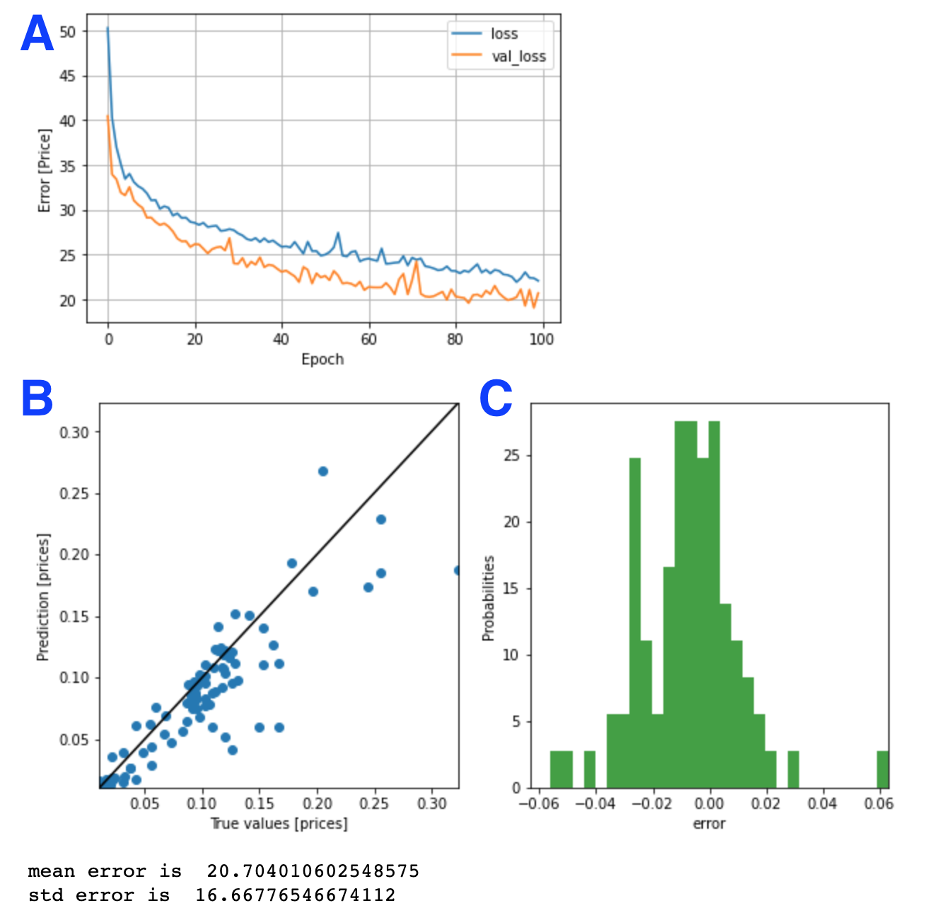
위의 결과에서 A는 train loss와 검증 loss의 변화를 보여준다. B와 C는 훈련이 끝난 모델을 검증 데이터로 평가한 결과를 보여준다. 평균적인 오차는 20.7%가 나왔다. 즉, 정확도는 약 80%이다. 꽤 괜찮은 정확도이다.
모델의 정확도 향상
1. Check skewness of target data
한 feature내의 데이터 분포의 왜곡정도(왜도, skewness)가 크면 모델의 정확도를 낮추는 결과를 초래한다. 이런 경우 데이터의 분표를 교정하여 skewness를 최소화 시켜주면 모델의 정확도를 높일 수 있다.
log(1+x)를 적용하면 데이터 분포의 극값들의 차이를 줄여 가우시안에 가깝게 분포를 변형시켜 준다. 이렇게 바뀐 분포는 최소의 skewness를 가진다.
from scipy import stats
from scipy.stats import norm, skew

def compare_skewness(inputDist1, inputDist2):
    plt.figure(figsize=(10,10))
    plt.subplot(2,2,1)
    sns.distplot(inputDist1 , fit=norm)
    plt.ylabel("Probability")
    (mu, sigma) = norm.fit(inputDist1)
    print( '\n InputDist1: mu = {:.2f} and sigma = {:.2f}'.format(mu, sigma))

    plt.subplot(2,2,2)
    res = stats.probplot(inputDist1, plot=plt)
    # Get the fitted parameters used by the function


    plt.subplot(2,2,3)
    sns.distplot(inputDist2 , fit=norm)
    plt.ylabel("Probability")
    (mu2, sigma2) = norm.fit(inputDist2)
    print( '\n InputDist2: mu = {:.2f} and sigma = {:.2f}\n'.format(mu2, sigma2))

    plt.subplot(2,2,4)
    res = stats.probplot(inputDist2, plot=plt)


inputDist1 = train["price"]
inputDist2 = np.log1p(train["price"])

compare_skewness(inputDist1, inputDist2)
2. Correct the target data
target 데이타 (house price)의 로그값을 취하고 규격화 시켜준다.
trainY = np.log1p(train["price"])
testY = np.log1p(test["price"])
maxPrice = max(max(trainY), max(testY))
trainY = trainY/maxPrice
testY = testY/maxPrice

plt.hist(trainY, bins=25,label="trainY")
plt.hist(testY, bins=25, label="testY")
plt.legend(loc='upper right')
plt.xlabel("normalized price")
plt.ylabel("occurrence")
plt.show()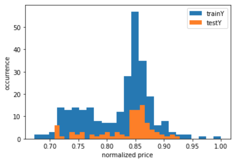
3. Train and evaluate model
모델을 다시 훈련시켜본다.
model = create_mlp(trainX.shape[1], regress=True)


print("[INFO] training model...")
history = model.fit(x=trainX,y=trainY,validation_data=(testX, testY),epochs=100, batch_size=8, verbose=0)

plot_loss(history)
prediction(testX, testY)
에러가 1.8까지 줄었고, 정확도는 98%까지 증가했다.
참고문헌
'Programming > Machine Learning' 카테고리의 다른 글
| 1D Convolutional Neural Network 이해하기 (CNN in numpy & keras) (0) | 2021.08.27 |
|---|---|
| Feature Importance with Information Gain (0) | 2021.08.21 |
| Seaborn boxplot으로 five-number summary 이해하기 (0) | 2021.05.03 |
| Information Gain (간단한 예제 & 파이썬 코드) (3) | 2020.12.12 |
| Tensorflow: regression 기본 예제 (연료 효율성 예측) (0) | 2020.11.14 |


댓글