[OpenCV] Difference of Gaussians(DoG)
이미지 처리에서 sharpening이라고 하는 즉 선명도를 증가시키는 방법이 몇 가지 있습니다. 가장 대표적인 방법으로 다음의 3가지를 뽑을 수 있고, 이 포스팅에선 두 개의 가우시안 분포의 차이로 얻는 방법을 보도록 하겠다.
- Laplace operator
- Difference of Gaussians (DoG)
- Unsharp Filter
2020/10/18 - [OpenCV] - [OpenCV] Image Edge Enhancement: 라플라스 연산자 (Laplace Operator)-파이썬 코드 포함
2020/10/27 - [OpenCV] - [OpenCV] 이미지 경계선 강화: Unsharped 필터 - 파이썬 코드 포함
Theory
$$ \begin{align} G_1(x,y) &= \frac{1}{\sqrt{2\pi\sigma_1^2}}\exp\left(-(x^2+y^2)/2\sigma_{1}^2\right)\tag{1}\\ G_2(x,y) &= \frac{1}{\sqrt{2\pi\sigma_2^2}}\exp\left(-(x^2+y^2)/2\sigma_{2}^2\right) \tag{2} \end{align} $$
These two Gaussian filter produces two blurred images. Difference of Gaussians is then made by subtracting more blurred image from less blurred one, ensuring that $\sigma_1 < \sigma_2$.
\begin{equation} f_{\mathrm{sharpened}}(x,y) = f(x,y)* G_1(x,y) - f(x,y) * G_2(x,y) \tag{3} \end{equation}
where $* $ indicates convolution operator.
The DoG curve resembles a Mexican hat as shown below.
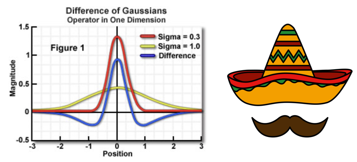
The resulting blue curve retains the location of maximum intensity, and surrounding of the location decreases to negative intensities in both sides, which makes the edge distinctive.
Python Code
import os
import cv2
import numpy as np
import matplotlib.pyplot as plt
import imghdr

class DoG:
    def __init__(self,file):
        # load a gif image
        if imghdr.what(file) == 'gif':
            gif = cv2.VideoCapture(file)
            ret, self.originalImage = gif.read()
        else:
            self.originalImage = cv2.imread(file)

    def DoG_by_OpenCV(self,kernel1,kernel2):
        self.src_gray = cv2.cvtColor(self.originalImage,cv2.COLOR_BGR2GRAY)
        self.G1_cv = cv2.GaussianBlur(self.src_gray,(kernel1,kernel1),0)
        self.G2_cv = cv2.GaussianBlur(self.src_gray,(kernel2,kernel2),0)
        self.DoG_cv = self.G1_cv.astype(np.float32) - self.G2_cv.astype(np.float32)

        self.sigma_1 = 0.3*((kernel1-1)*0.5-1) + 0.8
        self.sigma_2 = 0.3*((kernel2-1)*0.5-1) + 0.8

    def replicate_boundary(self,r_curr, c_curr,row,col):
        r_temp = r_curr
        c_temp = c_curr
        if r_temp<0:
            r_temp +=1
        elif r_temp>=row:
            r_temp -=1

        if c_temp<0:
            c_temp +=1
        elif c_temp>=col:
            c_temp -=1
        return r_temp, c_temp

    def get_GaussianBlurred(self,gkernel):
        row, col = self.src_gray.shape
        G = np.zeros((row,col))

        for r in range(row):
            for c in range(col):
                for i in range(3):
                    for j in range(3):
                        r_temp, c_temp = self.replicate_boundary(r+i-1,c+j-1,row,col)
                        G[r,c] += self.src_gray[r_temp,c_temp]*gkernel[i,j]

        return G

    def DoG_from_Scratches(self):
        xdir_gauss = cv2.getGaussianKernel(3, .5)
        gkernel1 = np.multiply(xdir_gauss.T, xdir_gauss)

        xdir_gauss = cv2.getGaussianKernel(3, 3.0)
        gkernel2 = np.multiply(xdir_gauss.T, xdir_gauss)

        self.G1_scratch = self.get_GaussianBlurred(gkernel1)
        self.G2_scratch = self.get_GaussianBlurred(gkernel2)
        self.DoG_scratch = self.G1_scratch-self.G2_scratch
a. 처리할 이미지 원본 그려보기
위 코드의 실행을 위해 아래의 원본 이미지를 다운받아서 입력 파일로 쓸 수 있다.
path = os.getcwd()
file = ''.join(path+"/wdg1.gif")
G = DoG(file)
plt.imshow(G.originalImage)
plt.title('Original Image',fontsize=15)
plt.xticks([]), plt.yticks([])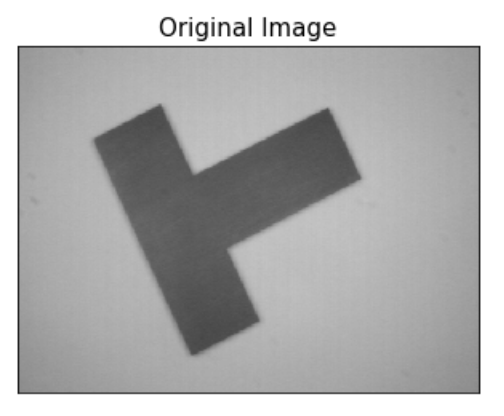
b. OpenCV에 의한 DoG 결과
G.DoG_by_OpenCV(3,5)

plt.figure(figsize=(20,6))
plt.subplot(131), plt.imshow(G.DoG_cv,cmap='gray'),plt.title('Resulting Image',fontsize=15)
plt.xticks([]), plt.yticks([])

plt.subplot(132), plt.imshow(G.G1_cv, cmap='gray'),plt.title('G1',fontsize=15)
plt.xticks([]), plt.yticks([])

plt.subplot(133), plt.imshow(G.G2_cv, cmap='gray'),plt.title('G2',fontsize=15)
plt.xticks([]), plt.yticks([])

print("sigma_1=",G.sigma_1)
print("sigma_1=",G.sigma_2)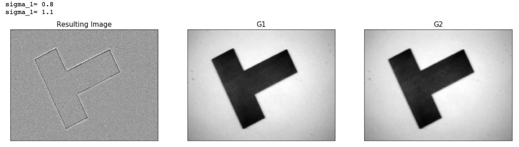
c. from-scratch DoG 결과
G.DoG_from_Scratches()

plt.figure(figsize=(20,6))
plt.subplot(131), plt.imshow(G.DoG_scratch,cmap='gray'),plt.title('Resulting Image',fontsize=15)
plt.xticks([]), plt.yticks([])

plt.subplot(132), plt.imshow(G.G1_scratch, cmap='gray'),plt.title('G1',fontsize=15)
plt.xticks([]), plt.yticks([])

plt.subplot(133), plt.imshow(G.G2_scratch, cmap='gray'),plt.title('G2',fontsize=15)
plt.xticks([]), plt.yticks([])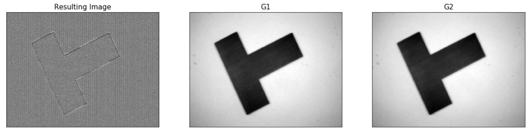
'Programming > Computer Vision' 카테고리의 다른 글
| [OpenCV] K-Means를 이용한 Image Segmentation(이미지 분할) (0) | 2020.11.05 |
|---|---|
| [OpenCV] Image Edge Enhancement: 라플라스 연산자 (Laplace Operator)-파이썬 코드 포함 (0) | 2020.11.04 |
| [OpenCV] 이미지 경계선 강화: Unsharp 필터 - 파이썬 코드 포함 (0) | 2020.11.04 |
| [OpenCV] 이미지 노출 융합 (exposure fusion) 이란? (1) | 2020.11.01 |
| [OpenCV] 이미지 blurring (smoothing) 처리 (0) | 2020.10.31 |


댓글