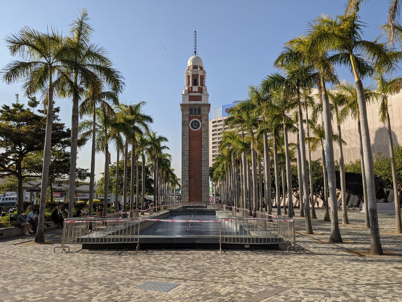
이미지 이진화(image binarization)는 아래의 도식에서 보이듯이 여러 이미지 분리(image segmentation)의 기법 중 가장 간단한 방법이다.
이진화라는 용어로부터 알 수 있듯이 이 방법은 이미지 픽셀의 여러 값들을 0 또는 255, 이를 테면 물체와 배경을 0과 255 혹은 그 반대의 방식으로, 이 두 값만으로 이미지의 모든 픽셀 값을 변환하는 것이다.
이 방법은 픽셀값이 0~255 사이의 값을 가지는 흑백 이미지에만 적용할 수 있다. 픽셀값을 0과 255만으로 바꾸기 위해 thresh라는 임계값을 먼저 정해야 한다. 임계값 보다 큰 픽셀은 모두 0 그렇지 않으면 모두 255 이런 식으로 픽셀값을 변환하는 것이다.
임계값을 수동으로 혹은 알고리즘에 의해 자동으로 설정할 수 있다. 수동으로 주는 것을 simple image thresholding이라고 하며, 자동으로 설정하는 알고리즘 중 가장 많이 사용되는 것은 Otus's method이다.
여기에서 이 두 방법으로 정해진 임계값을 기준으로 이미지 이진화를 실행해 보도록 하겠다.
Simple image thresholding
먼저 simple image thresholding으로 이미지 이진화를 해보도록 하자.
우선 필요한 모듈을 로딩하도록 한다.
import cv2
import numpy as np
import matplotlib.pyplot as plt
그리고 샘플 이미지를 읽어 변수에 저장하고 OpenCV의 라이브러리를 이용해서 이진화를 실행해본다. 여기에서 Thresh=0, 최대 픽셀값은 255로 주었다.
image = cv2.imread('threshold.png')

thresh = 0
maxValue = 255

th, dst = cv2.threshold(image, thresh, maxValue, cv2.THRESH_BINARY)

plt.figure(figsize=(10,5))
plt.subplot(121),plt.imshow(image, cmap='gray'),plt.title('original image',fontsize=15)
plt.xticks([]), plt.yticks([])

plt.subplot(122),plt.imshow(dst,cmap='gray'),plt.title('filtered image',fontsize=15)
plt.xticks([]), plt.yticks([])
아래 결과에서 보듯이 원본 이미지에는 식별하기 어려웠던 32,64, 5가 선명하게 보이는 것을 볼 수 있다. 그리고 숫자는 밝기가 255로 배경은 0으로 처리된 흑백 이미지 (binary image)가 되었다.

threshold값을 바꾸어 가며 이진화 결과를 확인해 볼 수 있다.
Otsu's algorithm
Otus 알고리즘은 thresh 값을 사용자 임의로 정하는 것이 아니라, 알고리즘 내에서 자동으로 정해지도록 하는 방법이다.
이 알고리즘의 기본적인 전제는 이미지가 bimodal distribution이라는 것이다. 즉, 이미지 픽셀값들의 히스토그램은 서로 다른 두 개의 픽셀값에서 최대값이 나타는 double peak 분포를 가진다는 것이다.
왼쪽 클래스의 피크는 배경 값, 오른쪽 클래스의 피크는 물체의 값일 것이다. 이 두 분포를 가장 잘 나누는 픽셀값을 찾는 것이 이 알고리즘의 핵심이다. 이 전제에 의거해 다음의 수식을 세울 수 있다.
\begin{equation} \sigma_{T}^2 = \sigma_w^2(t) + \sigma_b^2(t) \label{eq:totalVariance}\end{equation}
이것의 의미는 전체 분포의 분산 $\sigma_T$는 두 클래스 내의 (within-class) 분산($\sigma_w$)과 두 클래스 사이의 (between-class) 분산($\sigma_b$)으로 이루어져 있다는 것을 뜻한다.
\begin{equation} \sigma_w^2(t) = \omega_1(t)\sigma_1^2(t) + \omega_2(t)\sigma_2^2(t) \label{eq:withinClass}\end{equation}
두 클래스 사이의 분산 (between-class variance)은 다음과 같이 정의된다.
\begin{equation} \sigma_b^2(t) = \omega_1(t)\omega_2(t)\left[\mu_1(t)-\mu_2(t) \right]^2 \label{eq:betweenClass}\end{equation}
이때, 두 클래스의 경계값은 $\sigma_w$을 최소화 시킴과 동시에 $\sigma_b$를 최대화시키는 값으로 정해진다.
따라서 두 클래스 분포 중 하나를 선택해서 두 클래스를 가장 잘 구분하는 최적의 thresh값을 찾아내는 것이다. 주로 두 번째 Between-class 분포를 이용한다.
a. 이미지 로드와 히스토그램 측정
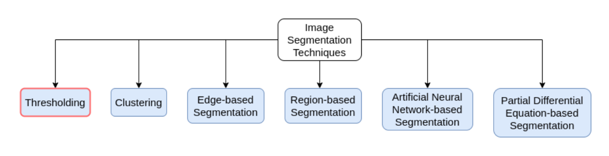
이 알고리즘의 핵심은 이미지의 히스토그램이고, 실행을 위해 새로운 흑백 이미지를 읽고 히스토그램을 만들어본다.
image = cv2.imread('boat_initial.jpg', 0)

hist, bin_edges = np.histogram(image, bins=256)

plt.figure(figsize=(14,5))
plt.subplot(121)
plt.imshow(image, cmap='gray')
plt.title('original image',fontsize=15)
plt.xticks([])
plt.yticks([])

plt.subplot(122),plt.plot(hist),plt.title('Histogram',fontsize=15)
아래 그림의 오른쪽에 히스토그램이 있다. 히스토그램의 높은 값들은 왼쪽 이미지의 밝은 값의 픽셀, 즉 배경으로부터 온 값이다. 반면 이미지에서 분리하고 싶은 부분은 물체에 해당하는 배와 그위의 사람들이다. 이 부분은 비교적 낮은 픽셀값들에 해당하며 그 픽셀의 수는 배경에 비해 아주 낮다.
b. Between-class variance를 최대화시키는 thresh값 찾기
weight1 = np.cumsum(hist)
weight2 = np.cumsum(hist[::-1])[::-1]

bin_mids = (bin_edges[:-1] + bin_edges[1:]) / 2.

mean1 = np.cumsum(hist * bin_mids) / weight1
mean2 = (np.cumsum((hist * bin_mids)[::-1]) / weight2[::-1])[::-1]

inter_class_variance = weight1[:-1] * weight2[1:] * (mean1[:-1] - mean2[1:]) ** 2
index_of_max_val = np.argmax(inter_class_variance)

threshold = bin_mids[:-1][index_of_max_val]

print("Otsu's algorithm implementation thresholding result: ", threshold)


# Plotting weight and between-class variance
plt.figure(figsize=(14,5))
plt.subplot(121)
plt.plot(weight1)
plt.plot(weight2)
plt.title('Weight profiles',fontsize=15)
plt.xlabel('pixel values'), plt.ylabel('weight')

plt.subplot(122)
plt.plot(inter_class_variance)
plt.title('Between-class variance',fontsize=15)
plt.xlabel('pixel values'), plt.ylabel('variance')
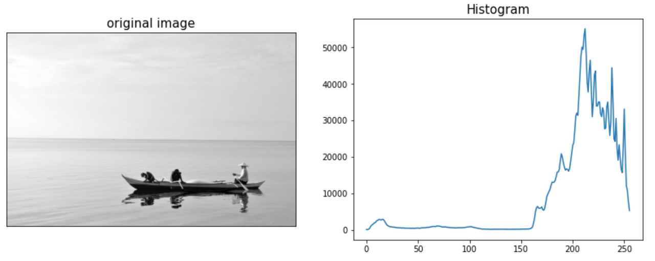
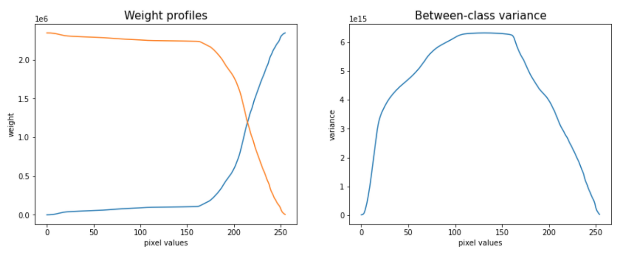
Between-class 분포에서, 각 클래스의 확률은 cumulative sum으로 양끝으로부터 축적된 값이 된다.
\begin{equation} \omega_1(t) = \sum_{i=0}^{t-1} p(i), \quad \omega_2(t) = \sum_{i=t}^{0} p(i) \label{eq:classProb} \end{equation}
즉, 높은 픽셀값을 가지는 픽셀들과 낮은 픽셀값을 가지는 픽셀값의 분포가 교차한다. 아래의 왼쪽 그림이 두 클래스의 분포의 비교를 보여주며, 이 두 클래스의 between-class의 분산이 가장 큰 곳이 바로 threshold값으로 지정할 수 있다.
c. OpenCV 내장 함수를 이용해서 얻은 thresh값과 비교
위의 코딩으로부터 얻은 경계값은 약 131.98, 이것은 OpenCV 라이브러리로 얻은 값과 비슷하다.
otsu_threshold, image_result = cv2.threshold(image, 0, 255, cv2.THRESH_BINARY + cv2.THRESH_OTSU)
print(otsu_threshold)

#132.0
d. 결과
이 경계값을 이용해 다음과 같이 이미지 이진화를 적용해본다. 결과 배와 사람들이 배경으로부터 잘 분리되었다.
th, dst = cv2.threshold(image, otsu_threshold, maxValue, cv2.THRESH_BINARY)

plt.figure(figsize=(14,5))
plt.subplot(121)
plt.imshow(image, cmap='gray')
plt.title('original image',fontsize=15)
plt.xticks([]), plt.yticks([])

plt.subplot(122)
plt.imshow(dst,cmap='gray')
plt.title('filtered image',fontsize=15)
plt.xticks([]), plt.yticks([])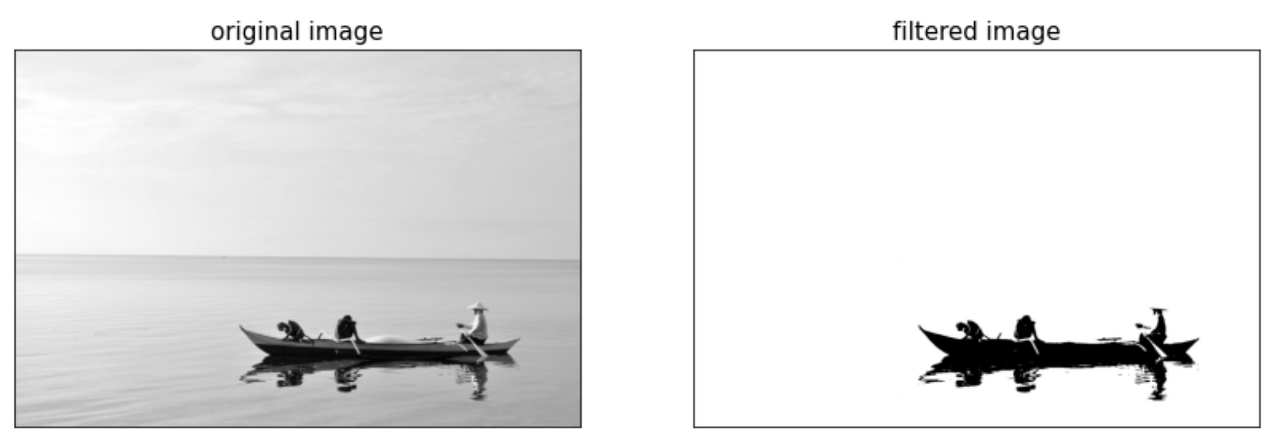
이진화된 이미지의 히스토그램 (histogram of binarized image)
hist_res, idx_res = np.histogram(dst, bins=256)
plt.plot(hist_res)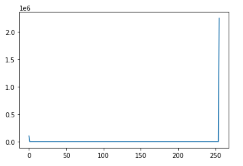
마치며
이번 포스팅에선 image segmentation의 기초적인 이미지 이진화 처리에 대해서 정리해 보았다. 이 방법은 주로 이미지의 전처리에 해당하며 Computer vision에서 중요한 기초이다. 임계값(thresh)을 찾아 픽셀값을 나누어 이미지의 픽셀값을 0과 255 두 그룹으로 양분하는 것이 핵심이다. 임계값은 주로 어림짐작으로 줄 수 있는 반면, Otus 알고리즘은 이미지 픽셀값들의 히스토그램을 이용해 자동으로 그 값을 찾는다. Otus알고리즘은 OpenCV에서 제공하니 바로 쉽게 적용할 수 있다.
References
'Programming > Computer Vision' 카테고리의 다른 글
| ValueError: matrix contains invalid numeric entries 에러 억제 방법 (Yolov5 + deepSORT) (0) | 2021.10.26 |
|---|---|
| FFMPEG로 다양한 input-output 소스 스트리밍하기 (option 설명 포함) (0) | 2021.10.23 |
| [OpenCV] K-Means를 이용한 Image Segmentation(이미지 분할) (0) | 2020.11.05 |
| [OpenCV] Image Edge Enhancement: 라플라스 연산자 (Laplace Operator)-파이썬 코드 포함 (0) | 2020.11.04 |
| [OpenCV] 이미지 경계선 강화: DoG - 파이썬 코드 포함 (0) | 2020.11.04 |


댓글